Binary Data

Paulo Fagandini

Nova SBE

Review

Review

We will need this:

\[ F = \frac{(R^2_{ur} - R^2_{r})/q}{(1 - R^2_{ur})/(n-k-1)} \]

Exercises

https://moodle.novasbe.pt/mod/folder/view.php?id=4021

Exercise 5.5

The players of a basketball team can play in three positions: guard, forward or center. The variable exper is the number of years as a professional player, points is the number of points scored per game, guard is a binary variable equal to one if the player is a guard and 0 otherwise, and forward is a binary variable equal to one if the player is a forward and 0 otherwise. Standard errors are reported in parentheses. Consider the following estimated equation:

\[ \widehat{points}= \underset{(1.18)}{4.76} + \underset{(0.33)}{1.28} exper - \underset{(0.024)}{0.072} exper^2 + \underset{(1.00)}{2.31}guard + \underset{(1.00)}{1.54}forward \] With \(n=269\), \(R^2=0.091\), \(\bar{R}^2=0.077\)

Question 5.5 a

Interpret the regression coefficients:

\[ \widehat{points}= \underset{(1.18)}{4.76} + \underset{(0.33)}{1.28} exper - \underset{(0.024)}{0.072} exper^2 + \underset{(1.00)}{2.31}guard + \underset{(1.00)}{1.54}forward \]

1. \(exper\)
2. \(guard\), \(forward\)

Note: It is not possible to interpret \(\hat{\beta}_1\) individually because it has no ceteris paribus interpretation: it is not possible to change experience holding squared experience fixed. Take the partial derivative of the dependent variable with respect to the independent variables.

The marginal impact of experience is given by \(1.28 − 2 × 0.071 exper\). Therefore, each additional year of experience increases the number of points scored per game at a decreasing rate (up until approximately 9 years of experience). For example: the fifth year increases the predicted number of points by \(1.28 - 2\times0.072\times4=0.704\), on average, ceteris paribus.

The players of a basketball team can play in three positions: guard, forward or center. Because center is not included in the model as a variable, it is the reference or comparison group.

Guard and forward are interpreted in comparison with the reference group, center. A guard player scores on average 2.31 more points per game relatively to a center player, ceteris paribus. A forward player scores on average 1.54 more points per game relatively to a center player, ceteris paribus.

Question 5.5 b

Why can’t we include in the model a binary variable center equal to one if the player is a center and zero otherwise?

\[ \widehat{points}= \underset{(1.18)}{4.76} + \underset{(0.33)}{1.28} exper - \underset{(0.024)}{0.072} exper^2 + \underset{(1.00)}{2.31}guard + \underset{(1.00)}{1.54}forward \]

1. \(exper\)
2. \(guard\), \(forward\)

Because of the dummy variables trap. It would introduce perfect collinearity in the model with intercept (each player plays in one of the three categories and the overall intercept (\(\beta_0\)) is for centers). \(guard=1−forward−center\). An alternative would be to include the three dummies excluding the intercept but then it would not be as straightforward to test differences between groups.

Question 5.5 c

Holding experience fixed, does a guard score more than a center? How much more? Is the difference statistically significant?

\[ \widehat{points}= \underset{(1.18)}{4.76} + \underset{(0.33)}{1.28} exper - \underset{(0.024)}{0.072} exper^2 + \underset{(1.00)}{2.31}guard + \underset{(1.00)}{1.54}forward \] With \(n=269\), \(R^2=0.091\), \(\bar{R}^2=0.077\)

A guard player is estimated to score on average 2.31 more points per game relatively to a center player, ceteris paribus. Is the difference statistically significant?

\[ H_0 : \beta_3 = 0\\ H_a : \beta_3 > 0 \]

The \(t\)-ratio equals \(2.31/1=2.31\) and the critical value for a one-tailed test with 5% significance level is \(t \sim t(269 − 4 − 1) = 1.645\). Therefore, we reject the null hypothesis.

Question 5.5 d

Considering also the following estimated equation, test if experience influences points.

\[ \widehat{points}= \underset{(1.18)}{4.76} + \underset{(0.33)}{1.28} exper - \underset{(0.024)}{0.072} exper^2 + \underset{(1.00)}{2.31}guard + \underset{(1.00)}{1.54}forward \]

With \(n=269\), \(R^2=0.091\), \(\bar{R}^2=0.077\)

\[ \widehat{points}= \underset{(0.86)}{8.52} + \underset{(1.03)}{2.40}guard + \underset{(1.03)}{1.68}forward \]

with \(n=269\) and \(R^2=0.020\), \(\bar{R}^2=0.012\)

\(H_0: \beta_1=0, \beta_2=0\), \(H_a: Not\ H_0\)

Then we can use an F-test:

\(F = [(0.091-0.020)/2]/[(1-0.091)/(269-4-1)]=10.31\)

The critical value \(F \sim F (2, 264)\) for a 5% significance level equals 3.00 and therefore we reject the null hypothesis.

Question 5.5 e

Consider a new equation with marital status (marr) as an additional explanatory variable:

\[ \widehat{points} = \underset{(1.18)}{4.70} + \underset{(0.33)}{1.23} exper - \underset{(0.02)}{0.07} exper^2 + \underset{(1.00)}{2.29} guard + \underset{(1.00)}{1.54} forward + \underset{(0.74)}{0.58} marr \]

Holding position and experience fixed, do married plyaers score more points?

\(H_0:\beta_5=0\), \(H_a: \beta_5>0\)

The t-ratio equals \(0.58/0.74=0.789\) and therefore for such a small value we fail to reject the null hypothesis.

Question 5.5 f

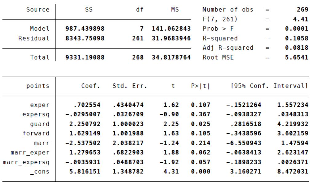
Consider the estimation output given in the table below for a new model that includes interactions of marital status with both experience variables. Is there strong evidence that marital status affects points per game?

Remember that we need to consider every variable that depends on the marital status variable.

\(H_0 : \beta_5 = \beta_6 = \beta_7 = 0\), \(H_a : Not\ H_0\)

To test this null hypothesis we compute an F-test:

\(F=[(0.1058−0.091)/(3)]/[(1−0.1058)/(269−7−1)]= 1.44\)

The \(F \sim F (3, 261)\) and therefore we fail to reject the null hypothesis in favor of the alternative hypothesis and there is no statistically significant evidence that marital status is important.

Question 5.5 g

Given this last estimated equation, what is the optimal number of years as a professional player if that player (for both married and not married players)?

We are looking for \((\partial \widehat{points})/(\partial exper)=0\)

If \(married=1\), \(0.70-2\times 0.0295\times exper + 1.28 - 2 \times 0.09 \times exper = 0 \Leftrightarrow exper^*=9.25\)

If \(married=0\), \(0.70-2\times 0.0295\times exper = 0 \Leftrightarrow exper^*=11.67\)

Question 5.9

Consider the following estimated equation:

\[ \widehat{sat}= \underset{(6.29)}{1029.10} + \underset{(3.83)}{19.30} hsize - \underset{(0.53)}{2.19} hsize^2 - \underset{(4.29)}{45.09} female - \underset{(12.71)}{169.81} black + \underset{(18.15)}{62.31} female\times black \] With \(n=4137\) and \(R^2=0.0858\).

The variable sat is the combined school average test (SAT) score, hsize is size of the student’s high school graduating class, in hundreds, female is a gender dummy variable, and black is a race dummy variable equal to one for black students and zero otherwise.

Question 5.9 a

Is there strong evidence that \(hsize^2\) should be included in the model? From this equation, what is the optimal high school size?

\[ \widehat{sat}= \underset{(6.29)}{1029.10} + \underset{(3.83)}{19.30} hsize - \underset{(0.53)}{2.19} hsize^2 - \underset{(4.29)}{45.09} female - \underset{(12.71)}{169.81} black + \underset{(18.15)}{62.31} female\times black \] With \(n=4137\) and \(R^2=0.0858\).

\(H_0:\beta_2=0\) and \(H_a: \beta\neq 0\).

The t-statistic equals \(t = − 2.19/0.53=-4.13\). For a 5% significance level and \((4, 137 − 5 − 1)\) degrees of freedom, the critical value is \(t_c = 1.96\). Because the \(|t|>|tc|\) we reject the null hypothesis.

What is the optimal high school size? This is a simple optimisation problem:\(\partial \widehat{sat}/\partial size = 0\)

\(19.3-2\times 2.19 \times hsize = 0 \Rightarrow hsize^*=4.41\)

Importantly, this means that the optimal school size is 4.41 hundreds of students, i.e., 441 students. [Remember that it is very important to look at the units of measurement of the variables]

Question 5.9 b

Holding hsize fixed what is the estimated difference in SAT score between nonblack females and nonblack males? How statistically significant is this estimated difference?

\[ \widehat{sat}= \underset{(6.29)}{1029.10} + \underset{(3.83)}{19.30} hsize - \underset{(0.53)}{2.19} hsize^2 - \underset{(4.29)}{45.09} female - \underset{(12.71)}{169.81} black + \underset{(18.15)}{62.31} female\times black \] With \(n=4137\) and \(R^2=0.0858\).

Let’s write the expected SAT score for the two groups holding \(hsize\) (and therefore \(hsize^2\) ) fixed:

\(E(sat|female = 1, black = 0) = \hat{\beta}_0 + \hat{\beta}_3\) (nonblack females)

\(E(sat|female = 0, black = 0) = \hat{\beta}_0\) (nonblack males)

Therefore, the estimated difference is \(\hat{beta}_3= −45.09\). Coefficient interpretation: The predicted SAT scores of nonblack females are on average 45.09 points lower than the SAT scores of nonblack males, on average, ceteris paribus. To test whether the difference between these two groups is statistically significant we consider the following null and alternative hypotheses:

\(H_0=\beta_3=0\) and \(H_a: \beta_3\neq 0\)

The t-statistic equals \(t=-45.09/4.29=-10.51\). For a 5% significance level (\(\alpha=5%\)) and (4,137-5-1) dof, the critical value is \(t_c=1.96\). Because \(|t|>|t_c|\) we reject the null, and \(\hat{\beta}_3\) is statistically significant.

Question 5.9 c

What is the estimated difference in SAT score between nonblack males and black males? Test the null hypothesis that there is no difference between their scores, against the alternative that there is a difference.

\[ \widehat{sat}= \underset{(6.29)}{1029.10} + \underset{(3.83)}{19.30} hsize - \underset{(0.53)}{2.19} hsize^2 - \underset{(4.29)}{45.09} female - \underset{(12.71)}{169.81} black + \underset{(18.15)}{62.31} female\times black \] With \(n=4137\) and \(R^2=0.0858\).

Let’s write the expected SAT score for the two groups holding \(hsize\) (and therefore \(hsize^2\) ) fixed: \(E(sat|female = 0, black = 1) = \hat{\beta}_0 + \hat{\beta}_4 (black males)\) \(E(sat|female = 0, black = 0) = \hat{\beta}_0 (nonblack males)\) Coefficient interpretation: on average, the predicted SAT scores of black males males are 169.81 points lower than the SAT scores of nonblack males, ceteris paribus. The null and alternative hypotheses are the following: \(H_0 : \beta_4 = 0\) and \(H_a : \beta_4 \neq 0\) respetively The t-statistic equals \(t = − 169.81/12.71=-13.36\). For a 5% significance level and (4, 137 − 12.715 − 1) degrees of freedom, the critical value is \(t_c = 1.96\). Because the \(|t| > |t_c|\) we reject the null hypothesis in favor of the alternative hypothesis and \(\hat{\beta}_4\) is individually statistically significant.

Question 5.9 d

What is the estimated difference in SAT score between black females and nonblack females? What would you need to do to test whether the difference is statistically significant?

\[ \widehat{sat}= \underset{(6.29)}{1029.10} + \underset{(3.83)}{19.30} hsize - \underset{(0.53)}{2.19} hsize^2 - \underset{(4.29)}{45.09} female - \underset{(12.71)}{169.81} black + \underset{(18.15)}{62.31} female\times black \] With \(n=4137\) and \(R^2=0.0858\).

\(E(sat|female = 1, black = 1) = \hat{\beta}_0 + \hat{\beta}_3 + \hat{\beta}_4 + \hat{\beta}_5\) (black females) \(E(sat|female = 1, black = 0) = \hat{\beta}_0 + \hat{\beta}_3\) (nonblack females)

The difference between the groups is \(\hat{\beta}_3+\hat{\beta}_4+\hat{\beta}_5−\hat{\beta}_3=\hat{\beta}_4+\hat{\beta}_5\). Then the null hypothesis can be written as \(H_0 : \beta_4 + \beta_5 = 0\)

Coefficient interpretation: According to the estimates, on average, the predicted SAT scores of black females are 107.5 points lower than the SAT scores of nonblack females, ceteris paribus.

The null and alternative hypotheses are the following: \(H_0:\beta_4+\beta_5=0\) and \(H_a:Not\ H_0\)

To test this null hypothesis using a t-statistic we would need the covariance between \(\hat{\beta}_4\) and \(\hat{\beta}_5\) : \(t=(\hat{\beta}_4+\hat{\beta}_5)/\sqrt{V[\hat{\beta}_4]+V[\hat{\beta}_5]+2Cov(\hat{\beta}_4,\hat{\beta}_5)}\)

Appendix

t table

df-\(\alpha/2\)	0.50	0.25	0.20	0.15	0.10	0.05	0.025	0.01	0.005	0.001	0.0005
1	0.000	1.000	1.376	1.963	3.078	6.314	12.71	31.82	63.66	318.31	636.62
2	0.000	0.816	1.061	1.386	1.886	2.920	4.303	6.965	9.925	22.327	31.599
3	0.000	0.765	0.978	1.250	1.638	2.353	3.182	4.541	5.841	10.215	12.924
4	0.000	0.741	0.941	1.190	1.533	2.132	2.776	3.747	4.604	7.173	8.610
5	0.000	0.727	0.920	1.156	1.476	2.015	2.571	3.365	4.032	5.893	6.869
6	0.000	0.718	0.906	1.134	1.440	1.943	2.447	3.143	3.707	5.208	5.959
7	0.000	0.711	0.896	1.119	1.415	1.895	2.365	2.998	3.499	4.785	5.408
8	0.000	0.706	0.889	1.108	1.397	1.860	2.306	2.896	3.355	4.501	5.041
9	0.000	0.703	0.883	1.100	1.383	1.833	2.262	2.821	3.250	4.297	4.781
10	0.000	0.700	0.879	1.093	1.372	1.812	2.228	2.764	3.169	4.144	4.587
11	0.000	0.697	0.876	1.088	1.363	1.796	2.201	2.718	3.106	4.025	4.437
12	0.000	0.695	0.873	1.083	1.356	1.782	2.179	2.681	3.055	3.930	4.318
13	0.000	0.694	0.870	1.079	1.350	1.771	2.160	2.650	3.012	3.852	4.221
14	0.000	0.692	0.868	1.076	1.345	1.761	2.145	2.624	2.977	3.787	4.140
15	0.000	0.691	0.866	1.074	1.341	1.753	2.131	2.602	2.947	3.733	4.073
16	0.000	0.690	0.865	1.071	1.337	1.746	2.120	2.583	2.921	3.686	4.015
17	0.000	0.689	0.863	1.069	1.333	1.740	2.110	2.567	2.898	3.646	3.965
18	0.000	0.688	0.862	1.067	1.330	1.734	2.101	2.552	2.878	3.610	3.922
19	0.000	0.688	0.861	1.066	1.328	1.729	2.093	2.539	2.861	3.579	3.883
20	0.000	0.687	0.860	1.064	1.325	1.725	2.086	2.528	2.845	3.552	3.850
21	0.000	0.686	0.859	1.063	1.323	1.721	2.080	2.518	2.831	3.527	3.819
22	0.000	0.686	0.858	1.061	1.321	1.717	2.074	2.508	2.819	3.505	3.792
23	0.000	0.685	0.858	1.060	1.319	1.714	2.069	2.500	2.807	3.485	3.768
24	0.000	0.685	0.857	1.059	1.318	1.711	2.064	2.492	2.797	3.467	3.745
25	0.000	0.684	0.856	1.058	1.316	1.708	2.060	2.485	2.787	3.450	3.725
26	0.000	0.684	0.856	1.058	1.315	1.706	2.056	2.479	2.779	3.435	3.707
27	0.000	0.684	0.855	1.057	1.314	1.703	2.052	2.473	2.771	3.421	3.690
28	0.000	0.683	0.855	1.056	1.313	1.701	2.048	2.467	2.763	3.408	3.674
29	0.000	0.683	0.854	1.055	1.311	1.699	2.045	2.462	2.756	3.396	3.659
30	0.000	0.683	0.854	1.055	1.310	1.697	2.042	2.457	2.750	3.385	3.646
40	0.000	0.681	0.851	1.050	1.303	1.684	2.021	2.423	2.704	3.307	3.551
60	0.000	0.679	0.848	1.045	1.296	1.671	2.000	2.390	2.660	3.232	3.460
80	0.000	0.678	0.846	1.043	1.292	1.664	1.990	2.374	2.639	3.195	3.416
100	0.000	0.677	0.845	1.042	1.290	1.660	1.984	2.364	2.626	3.174	3.390
1000	0.000	0.675	0.842	1.037	1.282	1.646	1.962	2.330	2.581	3.098	3.300
Z	0.000	0.674	0.842	1.036	1.282	1.645	1.960	2.326	2.576	3.090	3.291

F table

df2-α=0.05	1	2	3	4	5	6	7	8	9	10
1.000	161.448	199.500	215.707	224.583	230.162	233.986	236.768	238.883	240.543	241.882
2.000	18.513	19.000	19.164	19.247	19.296	19.330	19.353	19.371	19.385	19.396
3.000	10.128	9.552	9.277	9.117	9.013	8.941	8.887	8.845	8.812	8.786
4.000	7.709	6.944	6.591	6.388	6.256	6.163	6.094	6.041	5.999	5.964
5.000	6.608	5.786	5.409	5.192	5.050	4.950	4.876	4.818	4.772	4.735
6.000	5.987	5.143	4.757	4.534	4.387	4.284	4.207	4.147	4.099	4.060
7.000	5.591	4.737	4.347	4.120	3.972	3.866	3.787	3.726	3.677	3.637
8.000	5.318	4.459	4.066	3.838	3.687	3.581	3.500	3.438	3.388	3.347
9.000	5.117	4.256	3.863	3.633	3.482	3.374	3.293	3.230	3.179	3.137
10.000	4.965	4.103	3.708	3.478	3.326	3.217	3.135	3.072	3.020	2.978
11.000	4.844	3.982	3.587	3.357	3.204	3.095	3.012	2.948	2.896	2.854
12.000	4.747	3.885	3.490	3.259	3.106	2.996	2.913	2.849	2.796	2.753
13.000	4.667	3.806	3.411	3.179	3.025	2.915	2.832	2.767	2.714	2.671
14.000	4.600	3.739	3.344	3.112	2.958	2.848	2.764	2.699	2.646	2.602
15.000	4.543	3.682	3.287	3.056	2.901	2.790	2.707	2.641	2.588	2.544
16.000	4.494	3.634	3.239	3.007	2.852	2.741	2.657	2.591	2.538	2.494
17.000	4.451	3.592	3.197	2.965	2.810	2.699	2.614	2.548	2.494	2.450
18.000	4.414	3.555	3.160	2.928	2.773	2.661	2.577	2.510	2.456	2.412
19.000	4.381	3.522	3.127	2.895	2.740	2.628	2.544	2.477	2.423	2.378
20.000	4.351	3.493	3.098	2.866	2.711	2.599	2.514	2.447	2.393	2.348
21.000	4.325	3.467	3.072	2.840	2.685	2.573	2.488	2.420	2.366	2.321
22.000	4.301	3.443	3.049	2.817	2.661	2.549	2.464	2.397	2.342	2.297
23.000	4.279	3.422	3.028	2.796	2.640	2.528	2.442	2.375	2.320	2.275
24.000	4.260	3.403	3.009	2.776	2.621	2.508	2.423	2.355	2.300	2.255
25.000	4.242	3.385	2.991	2.759	2.603	2.490	2.405	2.337	2.282	2.236
26.000	4.225	3.369	2.975	2.743	2.587	2.474	2.388	2.321	2.265	2.220
27.000	4.210	3.354	2.960	2.728	2.572	2.459	2.373	2.305	2.250	2.204
28.000	4.196	3.340	2.947	2.714	2.558	2.445	2.359	2.291	2.236	2.190
29.000	4.183	3.328	2.934	2.701	2.545	2.432	2.346	2.278	2.223	2.177
30.000	4.171	3.316	2.922	2.690	2.534	2.421	2.334	2.266	2.211	2.165
40.000	4.085	3.232	2.839	2.606	2.449	2.336	2.249	2.180	2.124	2.077
60.000	4.001	3.150	2.758	2.525	2.368	2.254	2.167	2.097	2.040	1.993
120.000	3.920	3.072	2.680	2.447	2.290	2.175	2.087	2.016	1.959	1.910
1000000000.000	3.841	2.996	2.605	2.372	2.214	2.099	2.010	1.938	1.880	1.831