Fundamentals of
Game Theory
Prague University of Economics and Business
Faculty of Informatics and Statistics
Introduction
Core Bibliography
The core of the contents of this chapter takes as reference the book
📖 Strategies and Games: Theory and Practice by Prajit K. Dutta. 2001 MIT Press.
Strategic Form Games (CH3)
Strategic Form Games
We will focus the utilization of Strategic Form games to model simoultaneous games, and therefore the timing of the game becomes unnecessary. We will just need the set of players, their strategies, and the payoffs associated to any strategy profile.
Strategic Form Games
- Let’s name our players \(P1\) and \(P2\)
- Let \(S_i\) be the set of strategies available for player \(i\)
- Say \(\pi_i(s_1,s_2)\) be the payoff for player \(i\), with \(s_1\in S_1\) and \(s_2\in S2\).
Strategic Form Games
Suppose \(S_1=\{U,D\}\) and \(S_2=\{L,R\}\), the payoff matrix would be:
| 1\(\setminus\) 2 | \(L\) | \(R\) |
|---|---|---|
| \(U\) | \((\pi_1(U,L),\pi_2(U,L))\) | \((\pi_1(U,R),\pi_2(U,R))\) |
| \(D\) | \((\pi_1(D,L),\pi_2(D,L))\) | \((\pi_1(D,R),\pi_2(D,R))\) |
Important
The payoff for each player, depends on the strategy profile, that in each position on the table, is the same.
Strategic Form Games
What if we have more than 2 players, and strategies?
- If we have \(N\in\mathbb{N}\) players, we will index them: 1,2, \(\dots\), \(N\).
- Their strategy space is \(S_i\).
- A strategy profile is an ordered tuple \((s_1,s_2,\dots,s_N)\in S_1\times S_2\times\dots S_N\).
- \(\pi_i(s_1,\dots,s_N)\) represents the payoff for player \(i\), given the strategy profile \((s_1,s_2,\dots,s_N)\).
We can do better
Strategic Form Games
Given that the strategies of the other players (other than player \(i\)) are out player’s \(i\) control, we will summarize them as \(s_{-i}\). So we will write:
\[\pi_i(s_1,\dots,s_N) = \pi_i(s_i,s_{-i}) \]
And \(s_{-i}\) represents all chosen \(s_j\) when \(j\neq i\). We could say the other’s strategies in the current strategy profile.
The Prissoner’s Dilemma
This is a classical game, and this is a great opportunity to introduce it:
Two prissoners, Calvin and Klein, are hauled in for a suspected crime. The \(DA\) speaks to each prisoner separately, and tells them that she more or less has the evidence to convict them but they could make her work a little easier (and help themselves) if they confess to the crime. She offers each of them the following deal: “Confess to the crime, turn a witness for the State, and implicate the ohter guy, and you will do no time. Of course, your confession will be worth a lot less if the other guy confesses as well. I that case, you both go in for 5 years. If you do not confess, however, be aware that we will nail you with the other guy’s confession, and then you will do fifteen years. In the event that I cannot get a confession from either of you, I have enough evidence to put you both away for a year.”
Prajit K. Dutta’s version of this game, in the book Strategies and Games: Theory and Practice. MIT Press, 2001.
The Prissoner’s Dilemma
Note that this would be something like a reverse payoff matrix, as as a payoff we are writing down the years in prison, and most likely, the lower the number of years in prison, the better for both prissoners!
| Calvin - Klein | Confess | Not Confess |
|---|---|---|
| Confess | \((5,5)\) | \((0,15)\) |
| Not Confess | \((15,0)\) | \((1,1)\) |
We can turn this table into something more traditional, assuming that each year in prison, equals a payoff of -1.
The Prissoner’s Dilemma
| Calvin - Klein | Confess | Not Confess |
|---|---|---|
| Confess | \((-5,-5)\) | \((0,-15)\) |
| Not Confess | \((-15,0)\) | \((-1,-1)\) |
- Suppose Calvin thinks Klein will confess. In that case, Calvin would be much better confessing! (\(-5 > -15\)).
- Suppose Calvin thinks Klein will Not Confess. In that case, Calvin would also be much better off by confessing! (\(0 > -1\))
The Prissoner’s Dilemma
Symmetrically, these options are the same for Klein. Note that confess is a dominant strategy, because independently of what the other decides, confess always generates at least as much payoff as any alternative. You cannot improve over the payoff you can get with confess, no matter what your counterpart is doing.
Equivalence in the Extensive form
We said, these are simoultaneous games, but we do not need that both prissoner’s actually chose simoultaneously. It is enough that when one decide, the other does not know what the first prisoner’s chose.
Equivalence in the Extensive form
Think on the Rock-Paper-Scissors game. As both players can see each others hands, simultaneity is necessary.
Suppose now that we introduce a referee. One player tells secretely to the referee what her choice is (rock, paper, or scissors). Then the referee asks the other player, separately what is her own choice. Finally the referee can reveal if there is a winner or a draw. The game works just fine, even though one player played first.
Equivalence in the Extensive form
The key was that the player that played last, did not know what the other player played when she made her decision, and also that the first player, knew that they other player was unaware of her move by the time she made her decision.
Equivalence in the Extensive form
This is the Strategic or Normal form to represent this game:
| 1-2 | \(R\) | \(P\) | \(S\) |
|---|---|---|---|
| \(R\) | \((0,0)\) | \((-1,1)\) | \((1,-1)\) |
| \(P\) | \((1,-1)\) | \((0,0)\) | \((-1,1)\) |
| \(S\) | \((-1,1)\) | \((1,-1)\) | \((0,0)\) |
Equivalence in the Extensive form
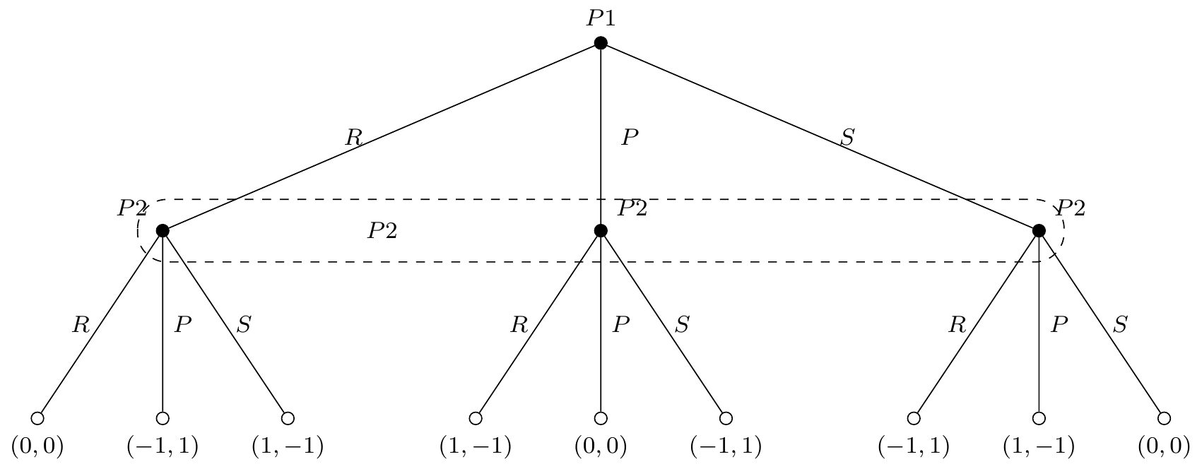
The dashed set represents an information set. This means that all these nodes carry the same information, or that at this point \(P2\) does not know exactly in which node she is, and must play accordingly. This is equivalent to a simoultaneous game.
Dominant Strategy Solution
Remember the dominan strategy in the Prissoner’s dilemma?
Confess was dominant, because no matter what the other player did, confessing always yielded the highest payoff.
Dominant Strategy Solution
Strongly Dominant Strategy
A strategy \(s_i'\) is said to be strongly dominant if \[\pi_i(s_i',s_{-i}) > \pi_i(s_i,s_{-i})\quad \forall s_i\in S_i,\ \forall s_{-i}\in\prod_{j\neq i} S_j\]
Dominant Strategy Solution
Weakly Dominant Strategy
A strategy \(s_i'\) is said to be weakly dominant if \[\pi_i(s_i',s_{-i})\geq \pi_i(s_i,s_{-i})\quad \forall s_i\in S_i,\ \forall s_{-i}\in\prod_{j\neq i} S_j\] and \[\exists \hat{s}_{-i}\in\prod_{j\neq i} S_j\ s.t.\ \forall s_i \in S_i\setminus\{s_i'\},\ \pi_i(s_i',\hat{s}_{-i})>\pi_i(s_i,\hat{s}_{-i})\]
Application: Second Price (Sealed Bid) Auctions
Suppose there is an auction, for which \(N\) bidders are competing. Each bidder \(i\) assigns a value \(v_i\) to the object being sold. The auction works like this:
- Every bidder submit a bid \(b_i\) in a sealed envelope.
- Once all bids are collected, the auctioneer opens the envelope, and announces the winner.
- The winner pays the value of the second highest bid, and gets the object. All other bidders walk out without the item, but without paying anything.
Application: Second Price Auctions
Any single bidder faces the following dilemma:
- If I bid too much, I will win for sure, but I might end up overpaying.
- If I bid too little, I will lose the auction and walk home empty handed.
Application: Second Price Auctions
- If the bidder gets the item, the payoff is \[\pi_i(b_i,b_{-i})=v_i-\max\{b_j\}_{j\neq i}\]
- If the bidder loses, the payoff is \[\pi_i(b_i,b_{-j})=0\]
- The expected payoff is then \[E\left[\pi_i(b_i,b_{-i})\right]=Pr\left(b_i>b_{-i}\right)\left(v_i-\max\{b_j\}_{j\neq i}\right)\]
Application: Second Price Auctions
The question is then, what is the value of \(b_i\) that maximizes the expected payoff? i.e. what is \(b_i^*\)?
- Suppose we chose \(b_i^*>v_i\).
- Suppose we choose \(b_i^*<v_i\).
- What about then if we choose \(b_i^*=v_i\)?
This is the solution proposed by William Vickrey, and these types of auctions are known as Vickrey Auctions.
Application: Second Price Auctions
These auctions present the bidder with some tradeoffs:
- Enforces true revelation (bidders reveal their true valuations).
- It is very simple and transparent.
- Might, under some reasonable assumptions, generate lower prices than other auction formats.
- Bidders might skip these auctions if they have reasons to hide their valuations from competitors.
Application: Second Price Auctions
Why now?
This auction presents an example of a dominant strategy, we saw that \(b_i=v_i\) always provides a higher (or equal) than any other bid, and therefore it is a weakly dominant strategy, whatever the other bidders are doing.
Dominance Solvability (CH 4)
Dominated Strategy
A strategy \(s_i^\#\in S_i\) is dominated by another strategy \(s_i'\in S_i\), if the latter does at least as well as \(s_i^\#\) against every strategy of the other players, and against some it does strictly better, such that:
\[\pi_i(s_i',s_{-i})\geq\pi_i(s_i^\#,s_{-i}),\quad \forall s_{-i}\in\prod_{j\neq i}S_j\] and \[\exists \hat{s}_{-i}\in\prod_{j\neq i} S_j,\ s.t.\ \pi_i(s_i',\hat{s}_{-i})>\pi_i(s_i^\#,\hat{s}_{-i})\]
If a strategy is not dominated, then it is said to be undominated.
Dominance Solvability
Corollary
If a strategy is dominated, it cannot be optimal.
Undominated vs Dominant strategy
Of course, looking at the definition, a dominant strategy is optimal, however, not every game has a dominant strategy for every player!
Dominance Solvability
How can we solve this problem?
Iterated Elimination of Dominated Strategies
A first approach to start looking for a solution, could be to reduce a game by removing dominated strategies, i.e. all the strategies for which there is always a better alternative whatever the other players chose to do.
Iterated Elimination of Dominated Strategies
Consider the following game
| P1 - P2 | Left | Right |
|---|---|---|
| Up | (1,1) | (0,1) |
| Middle | (0,2) | (1,0) |
| Down | (0,-1) | (0,0) |
- For \(P1\) there is no dominant strategy, but there is a dominated strategy, Down.
Iterated Elimination of Dominated Strategies
Consider the following game
| P1 - P2 | Left | Right |
|---|---|---|
| Up | (1,1) | (0,1) |
| Middle | (0,2) | (1,0) |
- For \(P2\) now, Right provides payoffs that are lower or equal than Left, and therefore it is dominated.
Iterated Elimination of Dominated Strategies
Consider the following game
| P1 - P2 | Left |
|---|---|
| Up | (1,1) |
| Middle | (0,2) |
- For \(P1\) now, Up is clearly the best choice, and the solution is therefore \((Up,Left)\). In this case it is said to be reached by iterated elimination of dominated strategies (IEDS). The game itself is said to be dominance solvable.
Nash Equilibrium (CH5)
Nash Equilibrium
So far we have discussed games in terms of “solutions,” but, what does that mean? What is an equilibrium in this framework?
Nash Equilibrium
- Suppose you know that strategy \(s_i\) is dominated by strategy \(s_i'\). Obviously you would chose \(s_i'\) every day of the week.
- Now, to chose some strategy \(s_i'\), you might need less than dominance. If you have some clue about what your opponent will do, then you just need to chose your strategy to maximize our payoff given what you expect the other players do, so you do not need to evaluate outcomes in unlikely scenarios.
Nash Equilibrium
Best Response
If given a fixed strategy profile \(\bar{s}_{-i}\in \prod_{j\neq i}S_j\) from the other players, \(s_i'\in S_i\) is the best response of player \(i\) if \[\pi_i(s_i',\bar{s}_{-i})\geq \pi_i(s_i,\bar{s}_{-i})\] for any \(s_i\in S_i\).
Is this enough to have an equilibrium?
Nash Equilibrium
No! Every single player needs to be best responding.
Nash Equilibrium
The strategy profile \(s^*=(s_1^*,s_2^*,\dots,s_N^*)\in S_1\times S_2 \times \dots \times S_N\) is a Nash Equilibrium if
\[\pi_i(s_i^*,s_{-i}^*)\geq \pi_i(s_i,s_{-i}^*),\quad \forall s_i\in S_i,\ \forall i\in \{1,\dots,N\}\]
Every \(s_k^*\) is itself a best response to \(s_{-k}^*\), and then, nobody has incentives to unilaterally change their decision.
Nash Equilibrium
Let’s check the proposed solution we found using IEDS for the game:
| P1 - P2 | Left | Right |
|---|---|---|
| Up | (1,1) | (0,1) |
| Middle | (0,2) | (1,0) |
| Down | (0,-1) | (0,0) |
\((Up,Left)\) is indeed a Nash Equilibrium, as every player is best responding, or no player can unilaterally profit from deviating from the NE.
Nash Equilibrium
Proposition
If in a game there is an outcome to IEDS. Then this outcome is a Nash Equilibrium. However, a Nash Equilibrium not always can be reached using IEDS.
We just saw an example of a IEDS where it was a NE. Let’s check an example where we have a NE that is not IEDS reachable.
Nash Equilibrium
There is classical game known as the Coordination game. Suppose two friends want to meet to catch up. They decide to go to some concert at 19:30.
| P1-P2 | 19:30 | 17:30 |
|---|---|---|
| 19:30 | (1,1) | (0,0) |
| 17:30 | (0,0) | (0,0) |
- What are the NE of this game?
- What is the solution using IEDS?
Application: The Tragedy of the Commons (CH7)
The tragedy of the Commons
“That which is common to the greatest number has the least care bestowed upon it. Everyone thinks chiefly of his own, hardly at all of the common interest.”
— Aristotle, Politics, II.3

The tragedy of the Commons
Even though this problem has been thought by thinkers since many millenia, it was formalize much more recently.
- The commons were lands shared in the center of 16th Century England villages, where, among other things, people could take their cattle pasture.
- In modern times we can find an example in International Waters, or the Athmosphere.
The tragedy of the Commons
They have two core features:
- Access to (almost) everybody
- Resource depletability (finite)
This indeed has the same core as the classical externality problem, this is what we will study.
The tragedy of the Commons
Intuition
Suppose you own a factory and you dump the fumes of your furnaces directly to the athmosphere.
- If you live in the area, you and eveyrone that lives around your factory will suffer (pay the costs) of your pollution.
- Given the cost is spread among many agents, you will overpollute, as well as any other factory in the area.
- Overall there will be a larger pollution level than the optimal for the local population.
The tragedy of the Commons
Let’s introduce a model to study this problem:
- Assume there are only two periods \(t=0,1\).
- Player \(i\) in period \(t\) consumes \(c_i^t\) with \(i=1,2\).
- Common property resource of size \(y^0>0\).
- \(y^1=y^0-\sum_{i\in\{1,2\}} c_i^0\).
- If they try to consume more than \(y^t\), in a single period, then each gets \(\frac{y^t}{2}\), and \(y^{t+1}=0\).
- Agents drive utility \(u(c)\) from consuming, with \(u'(c)>0\) and \(u''(c)<0\), for example \(u(c)=\ln(c)\).
The tragedy of the Commons
To solve this, we will use a technique that we will revisit in the future with more detailed, which is known Backward Induction. This means we will solve the problem starting from the end:
- If there is no \(t=2\), then consumers will try to consume as much as they can in \(t=1\), and therefore \(c_1=c_2=\frac{y^1}{2}\).
- Note that \(y^1=y^0-c_1^0-c_2^0\), and therefore \(c_i=\frac{y^0-c_1^0-c_2^0}{2}\) with \(i=1,2\).
Note that \(c_1^1\) and \(c_2^2\) are equal and depend on \(c_1^0\) and \(c_2^0\), and actually these are the only relevant variables. Let’s drop the supra-index for time.
The tragedy of the Commons
Let’s solve for consumer 1 (the problem is symmetric). Let’s take \(\bar{c}_2\) as “some” value for \(c_2\).
\[\max_{c_1} \ln(c_1)+\ln\left(\frac{y-c_1-\bar{c}_2}{2}\right)\]
From where deriving first order conditions we obtain:
\[\frac{1}{c_1}-\frac{1}{y-c_1-\bar{c}_2}=0\quad\Rightarrow\quad c_1=\frac{y-\bar{c}_2}{2}\]
The tragedy of the Commons
What we have here is, that if player 2 choses to consume \(\bar{c}_2\) in the first period, then player 1 will chose to consume \(\frac{y-\bar{c}_2}{2}\). Because the problem is symmetric, if we repeat the exercise, but now from the point of view of player 2, we will get \[c_2=\frac{y-\bar{c}_1}{2}\]
These are the best response functions of players 1 and 2. We know that both players should be best responding at the same time in a Nash Equilibrium.
The tragedy of the Commons
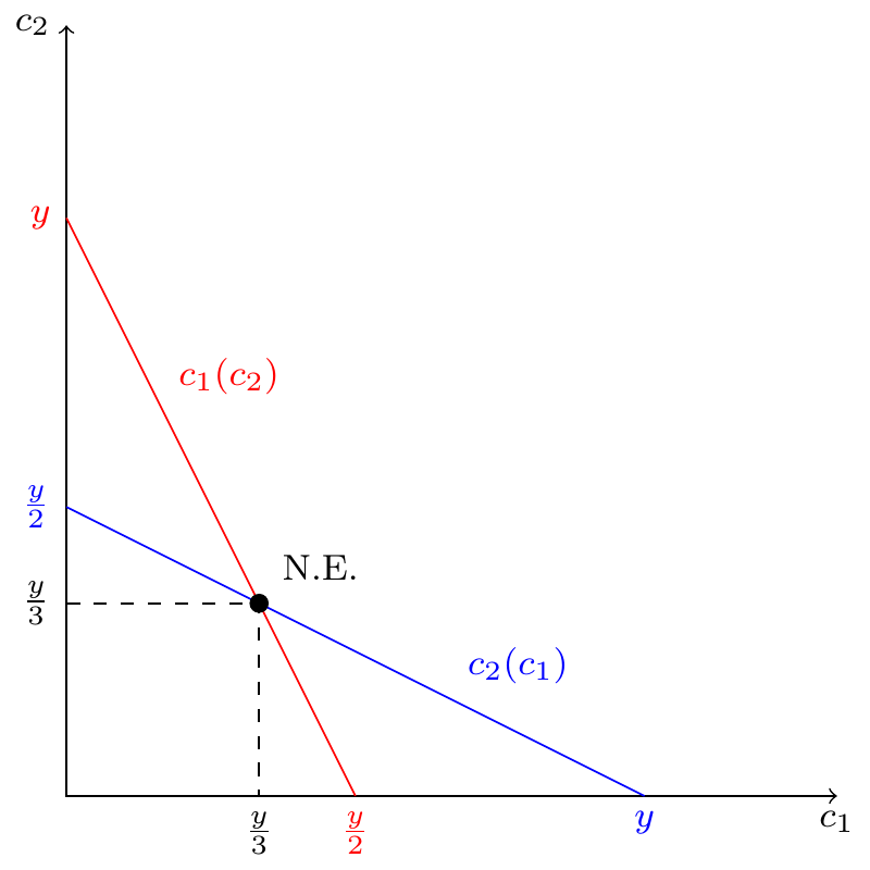
We get the following system of equations:
\[c_1^*=\frac{y-c_2^*}{2} \quad \text{and} \quad c_2^*=\frac{y-c_1^*}{2}\]
For example
\[c_1^*=\frac{y-\frac{y-c_1^*}{2}}{2}=\frac{y}{4}+\frac{c_1^*}{4}\ \Rightarrow\ c_1^*=\frac{y}{3}\]
By symmetry, \(c_2^*=\frac{y}{3}\).
The tragedy of the Commons
What we have then, is that both consumers will consume \(\frac{y}{3}\) in the first period and \(\frac{y}{6}\) in the second period. Their lifetime utility will be \(\ln \left(\frac{y}{3}\right)+\ln\left(\frac{y}{6}\right)=\ln\left(\frac{y^2}{18}\right)\). This is a Nash Equilibrium, because both players are best-responding.
The tragedy of the Commons
Is this socially optimal?
Social Optimum
A pattern of consumption, \((\hat{c}_1,\hat{c}_2)\) is socially optimal if it maximizes the sum of the two player’s utility, that is, if it solves the following problem:
\[\max_{c_1,c_2} \ln (c_1) + \ln (c_2) + 2 \ln \left(\frac{y-(c_1+c_2)}{2}\right)\]
The tragedy of the Commons
This leads to the first order conditions:
\[\frac{1}{c_1^*}-\frac{2}{y-c_1^*-c_2^*}=0\quad\text{and}\quad\frac{1}{c_2^*}-\frac{2}{y-c_1^*-c_2^*}=0\]
And solutions \(c_1^*=c_2^*=c^*\), and replacing in either equation, we obtain \(c^*=\frac{y}{4}\). Lifetime utility is \[2\ln \left(\frac{y}{4}\right)=\ln\left(\frac{y^2}{16}\right)>\ln\left(\frac{y^2}{18}\right)\]
The tragedy of the Commons
We can see the The tragedy of the Commons in action, the Nash Equilibrium leads to overconsumption in the first period and therefore to a lower level of lifetime utility.
Note:
- If player 1, for example, would try to cut consumption in the first period to “save” for the future,
- player 2 would consume now half more (look at the BRF),
- and in the second period, consumer 1 would have to split the savings (just half of his consumption reduction) with player 2.
The tragedy of the Commons
Graphical representation:
Mixed Strategies (CH8)
Mixed Strategies
Consider the game of Rock-Paper-Scissors. You have three possible strategies: {✊, ✋, ✌️}. So far we have considered that a strategy for you, would be to pick either of those options. You would think à priori that you have only 3 options, however, there are other options.
Mixed Strategies
What about if you would randomize your choice? For example, you could say that you will not play ✋ but you could play ✊ or ✌️. To decide which will be your choice, you will toss a coin 🪙.
- If you see head, you will chose ✊, and
- if you see tails you will choose ✌️.
Now you see, instead of having only three options, you have 4!
Mixed Strategies
Really you won an infinity of new possiblities, as any randomization would yield a new strategies. These are known as mixed strategies, when your strategy is to decide a probability distribution over the available actions.
Mixed Strategies
Definition
A strategy \(s^j\) is called a pure strategy, if, it contains a specific, concrete, and unambiguous, action for every decision node the agent might encounter along the game.
Definition
Suppose a player has \(M\) pure strategies \(s^1, s^2,\dots, s^M\). A mixed strategy for this player is a probability distribution over his pure strategies; that is, it is a probability vector \((p^1, p^2,\dots, p^M)\), with \(p^k\geq 0\), \(k=1,\dots,M\), and \(\sum_{k=1}^M p^k=1\).
Mixed Strategies
You could say that any pure strategy is a mixed strategy that concentrates the probability over a single strategy.
The pure strategy ✌️ is the same as the mixed strategy \(\{0,0,1\}\) over the pure strategies (✊,✋,✌️).
A reasonable question is, and then, how do we evaluate the payoffs?
Mixed Strategies
We use the expected payoffs. Consider the following game:
| P1 - P2 | Left | Right |
|---|---|---|
| Up | (3,1) | (0,0) |
| Down | (0,0) | (1,3) |
What Happens if \(P1\) randomizes \(\frac{2}{3}\) for Up, and \(P2\) plays for sure \(Left\)?
- For Player 1: \(E[\pi_1] = \frac{2}{3} 3 + \frac{1}{3} 0 = 2\)
- For Player 2: \(E[\pi_2] = \frac{2}{3} 1 + \frac{1}{3} 0 = \frac{2}{3}\)
Mixed Strategies
| P1 - P2 | Left | Right |
|---|---|---|
| Up | (3,1) | (0,0) |
| Down | (0,0) | (1,3) |
What if both players randomize? Suppose \(P1\) repeats her strategy, and \(P2\) now randomizes with 50% on each alternative.
- For Player 1: \(E[\pi_1]= \frac{2}{3}\frac{1}{2}3 + \frac{2}{3}\frac{1}{2}0 + \frac{1}{3}\frac{1}{2}0 + \frac{1}{3}\frac{1}{2}1 = \frac{7}{6}\)
- For Player 2: \(E[\pi_2]= \frac{2}{3}\frac{1}{2}1 + \frac{2}{3}\frac{1}{2}0 + \frac{1}{3}\frac{1}{2}0 + \frac{1}{3}\frac{1}{2}3 = \frac{5}{6}\)
Mixed Strategies
Definition
Suppose that player \(i\) plays a mixed strategy \((p^1,p^2,\dots,p^M)\). Suppose that the other players play the pure strategy \(s_{-i}^\#\). Then the expected payoff to player \(i\) is equal to \[E[\pi_i]= \sum_{k=1}^M p^k \pi_i(s^k,s_{-i}^\#)\]
Mixed Strategies
Proposition
- A mixed strategy \((p^1,\dots,p^M)\) is a best response to \(s_{-i}^\#\) if and only if each of the pure strategies in its support is itself a bset response to \(s_{-i}^\#\).
- In that case, any mixed strategy over the same support (strategies with positive probability), is a best response as well.
Note that if this is not the case, then you could drop the worse strategies and the expected payoff would increase!
Mixed Strategies
Fact
A mixed strategy can dominate some pure strategies.
| P1-P2 | L | \(M_1\) | \(M_2\) | R |
|---|---|---|---|---|
| U | (1,0) | (4,2) | (2,4) | (3,1) |
| M | (2,4) | (2,0) | (2,2) | (2,1) |
| D | (4,2) | (1,4) | (2,0) | (3,1) |
- No dominant strategy in pure strategies
- Suppose \(P1\) plays \(\left(\frac{1}{2},0,\frac{1}{2}\right)\).
Mixed Strategies
Expected payoffs for \(P1\) are:
\[[2.5, 2.5, 2, 3]\]
With this strategy, \(P1\) can ensure an expected payoff of \(2\) or more. This mixed strategy weakly dominates the pure strategy \(M\).
Does this change something on a solution in dominant strategy?
Mixed Strategies and NE
Without mixed strategies, there might be no NE, recall the game {✊, ✋, ✌️}. In every strategy profile, there are incentives for unilateral deviations!
| P1-P2 | ✊ | ✋ | ✌️ |
|---|---|---|---|
| ✊ | (0,0) | (-1,1) | (1,-1) |
| ✋ | (1,-1) | (0,0) | (-1,1) |
| ✌️ | (-1,1) | (1,-1) | (0,0) |
Mixed Strategies and NE
We know that if we would like to find a NE, we need that every player is best-responding, i.e., given the move of the other player, there is no way to improve.
This can only happen if any pure strategy in the support of the player, has the same expected payoff. If this is not the case, then the player has incentive to deviate to put a higher weight into the strategies with higher payoffs to increase her expected payoff.
Mixed Strategies and NE
Let’s consider a simpler game, to ease the computations. Suppose two friends attemp some penalty kicks, and let’s assume that there are only two options, Left or Right.
| P1 - P2 | Left | Right |
|---|---|---|
| Left | (-1,1) | (1,-1) |
| Right | (1, -1) | (-1, 1) |
In this game \(P2\) is the goalkeeper. We can see that this game has no NE in pure strategies as at least one player has always incentives to deviate.
Mixed Strategies and NE
Suppose \(P2\) will choose \(L\) with probability \(q\) and \(R\) with probability \((1-q)\).
What is the expected payoff for \(P1\)?
\[E[\pi_1|Left]=-1\times q + 1 \times (1-q) = 1-2q\] \[E[\pi_1|Right]=1\times q - 1 \times (1-q) = -1+2q\]
Mixed Strategies and NE
If one is larger than the other, then \(P1\) would surely choose that one, so in order to randomize as well, both must be equal:
\[1-2q=-1+2q\ \Rightarrow\ q=\frac{1}{2}\]
Now, if \(P2\) is randomizing, it must be true that the expected payoff of each pure strategy is also the same for her:
Mixed Strategies and NE
Suppose \(P1\) chooses Left with probability \(p\), and Right with probability \(1-p\):
\[E[\pi_2|Left]=1\times p - 1 \times (1-p) = -1+2p\] \[E[\pi_2|Right]=-1\times p + 1 \times (1-p) = 1-2p\]
And then, for \(P2\) randomize her decision, both must be equal, and so:
\[-1+2p=1-2p\quad\Rightarrow\quad p=\frac{1}{2}\]
Mixed Strategies and NE
The Nash Equilibrium in Mixed Strategies in this case is \(\left((L,p=\frac{1}{2}),(L,q=\frac{1}{2})\right)\).
Theorem (Nash)
In a game where mixed strategies are allowed, then every game with a finite number of players in which each player can choose from finitely many pure strategies has at least one Nash equilibrium, which might be in mixed or pure strategies.
Bibliography
Bibliography
These slides took definitions and examples from the book:
Strategies and Games: Theory and Applications from Prajit Dutta. 2001 MIT Press. Chapters 3-5 and 6-8. The expected payoff for \(P1\) is:

Economics of Incentives